Written by the CSCmotion Motion Control Engineering Team
Published: October 24, 2026 · Updated: October 24, 2026
Review scope: geometric derivation, synthetic numerical consistency, model assumptions and physical interpretation. Formula review by an engineer remains pending.
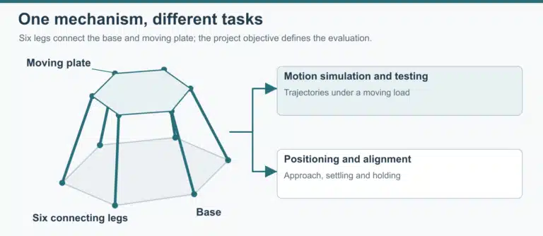
Stewart platform kinematics equations connect the position and orientation of a moving plate to the lengths of six legs. For inverse kinematics, transform each upper attachment point into the base coordinate frame, subtract its lower attachment point, and calculate the resulting vector’s length. Forward kinematics reverses that task: six known lengths constrain an unknown platform pose through coupled nonlinear equations.
The distinction becomes useful when a simulation appears to work but its output does not match a platform’s coordinate definition or actuator readings. A correct distance calculation can still use the wrong attachment order, reference height, rotation convention, or length zero. Establish those inputs before comparing solver results.
Coordinate Frames and the Six Leg Vectors
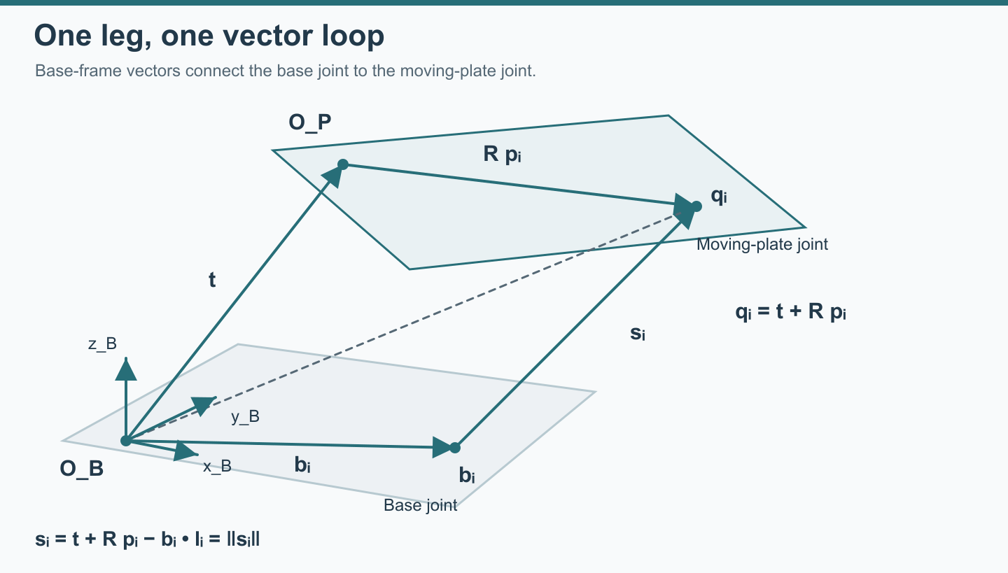
Use two coordinate frames: one fixed to the base and one fixed to the moving plate. The attachment coordinates remain constant in their respective frames. The plate’s pose tells you how to transform between them. All terms in a leg vector must ultimately be expressed in the same frame.
Scroll horizontally to view all columns →
| Symbol | Meaning | Frame or unit |
|---|---|---|
| bᵢ | Lower attachment point for leg i | Base frame; mm in this example |
| pᵢ | Upper attachment point for the same leg | Moving-plate frame; mm |
| t | Position of the moving-frame origin | Base frame; mm |
| R | Rotation from moving-frame coordinates into base-frame coordinates | Dimensionless 3 × 3 matrix |
| qᵢ | Upper attachment point after transformation | Base frame; qᵢ = t + R pᵢ |
| sᵢ | Vector from the lower joint center to the upper joint center | Base frame; sᵢ = qᵢ − bᵢ |
| lᵢ | Distance between those two joint centers | lᵢ = ‖sᵢ‖; mm |
The index i runs from 1 to 6. It identifies a physical leg connection, not simply the next point around either circle. A different pairing of upper and lower points defines a different mechanism even if both circles have the same radius.
These definitions give the central relationship:
Scroll horizontally to read the full equation →
qᵢ = t + R pᵢ
sᵢ = t + R pᵢ − bᵢ
lᵢ = √(sᵢₓ² + sᵢᵧ² + sᵢ𝓏²)
The fixed-distance constraint is also the starting point of the general Stewart–Gough forward-kinematics formulation. It remains useful whether the solver stores orientation as angles, a rotation matrix, or a quaternion.
Read the orientation as a transformation
The example uses column vectors and R = R𝓏(γ) Rᵧ(β) Rₓ(α), with the rightmost rotation applied first.
Writing cα = cos α and sα = sin α, and similarly for β and γ, gives:
Scroll horizontally to view all columns →
| R row | Column 1 | Column 2 | Column 3 |
|---|---|---|---|
| 1 | cγ cβ | cγ sβ sα − sγ cα | cγ sβ cα + sγ sα |
| 2 | sγ cβ | sγ sβ sα + cγ cα | sγ sβ cα − cγ sα |
| 3 | −sβ | cβ sα | cβ cα |
Angles in the example tables are degrees; trigonometric calculations use their radian equivalents. Reordering the rotations generally changes R. Replacing R with its transpose reverses the coordinate transformation. Neither change is harmless when comparing two models.
Translations are sometimes labeled surge, sway, and heave in motion simulation. Roll, pitch, yaw describe orientation conventions. Record how those names map to the chosen axes, including signs and the reference point.
Also distinguish the moving-frame origin from the payload center of gravity or a desired pivot point. They can coincide in a particular model, but they are different definitions. A rigid offset from the plate origin transforms with the plate; it cannot simply be added as a fixed base-frame offset after every rotation. For the mechanism and layout choices behind these coordinates, see Stewart platform design.
Inverse Kinematics: One Pose, Six Leg Lengths
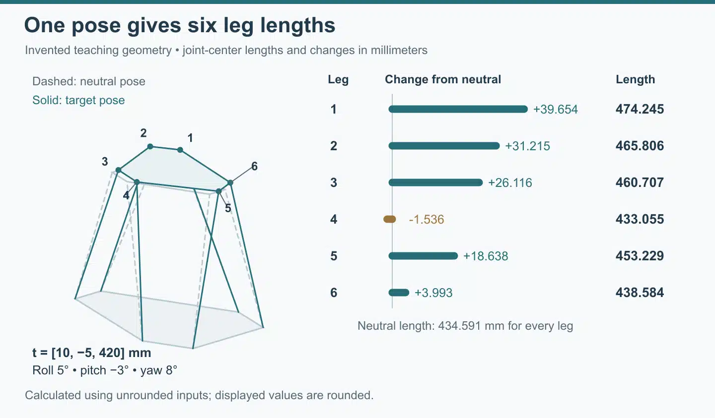
Once the attachment coordinates and pose are fixed, inverse kinematics is a distance calculation for each leg. Rotation moves the upper attachment relative to the moving-frame origin; translation places that origin in the base frame. Subtract the lower attachment only after applying both operations.
Taking the dot product of the leg vector with itself gives:
Scroll horizontally to read the full equation →
lᵢ² = (t + R pᵢ − bᵢ)ᵀ(t + R pᵢ − bᵢ)
Since RᵀR = I for a rotation matrix, the same expression can be expanded as:
Scroll horizontally to read the full equation →
lᵢ² = tᵀt + pᵢᵀpᵢ + bᵢᵀbᵢ + 2tᵀR pᵢ − 2tᵀbᵢ − 2bᵢᵀR pᵢ
Take the nonnegative square root to obtain length. The compact vector form is easier to inspect; the expanded form provides a separate algebraic check. Both describe the same joint-center distance. The kinematic study’s inverse-kinematics section also distinguishes total leg length from its change relative to an initial configuration.
Define a complete teaching geometry
The worked example uses invented teaching dimensions, not a CSCmotion platform configuration.
Choose a base attachment radius of 300 mm and a moving-plate attachment radius of 180 mm. All lower points have base-frame z = 0, and all upper points have moving-frame z = 0. Use the angle pairs below, measured counterclockwise from positive x toward positive y in each frame.
For each row, compute bᵢ = (300 cos θᵢ, 300 sin θᵢ, 0) and pᵢ = (180 cos φᵢ, 180 sin φᵢ, 0). The angle definitions, rather than the rounded coordinates, are the reproducible inputs.
Scroll horizontally to view all columns →
| Leg | θᵢ, base angle | φᵢ, upper angle | bᵢ: x, y in mm | pᵢ: x, y in mm |
|---|---|---|---|---|
| 1 | 15° | 45° | 289.778, 77.646 | 127.279, 127.279 |
| 2 | 105° | 75° | −77.646, 289.778 | 46.587, 173.867 |
| 3 | 135° | 165° | −212.132, 212.132 | −173.867, 46.587 |
| 4 | 225° | 195° | −212.132, −212.132 | −173.867, −46.587 |
| 5 | 255° | 285° | −77.646, −289.778 | 46.587, −173.867 |
| 6 | 345° | 315° | 289.778, −77.646 | 127.279, −127.279 |
At the reference pose, let t₀ = (0, 0, 400) mm and R₀ = I. Each paired attachment has an angular difference of either +30° or −30°, so every reference length is:
Scroll horizontally to read the full equation →
lᵢ₀ = √(300² + 180² − 2 × 300 × 180 × cos 30° + 400²) = 434.591 mm, rounded.
That equal-length result is a useful check for this geometry. Changing anchor positions, plate offsets, or the reference pose changes the reference lengths.
Apply a mixed translation and rotation
Set the target origin to t = (10, −5, 420) mm. Use roll α = 5°, pitch β = −3°, and yaw γ = 8°, with the matrix order defined above. Evaluating R gives:
Scroll horizontally to view all columns →
| R row | Column 1 | Column 2 | Column 3 |
|---|---|---|---|
| 1 | 0.988911 | −0.143160 | −0.039500 |
| 2 | 0.138982 | 0.985865 | −0.093564 |
| 3 | 0.052336 | 0.087036 | 0.994829 |
For leg 1, first rotate p₁, then add t and subtract b₁. The resulting leg vector is approximately (−172.131, 60.524, 437.739) mm. Its length is therefore:
Scroll horizontally to read the full equation →
l₁ = ‖s₁‖ ≈ 474.245 mm
Calculated using unrounded inputs; the displayed vector components are rounded.
Repeating the same operation for all six legs gives the following calculated example. Values are rounded to three decimal places for readability; calculations use the unrounded coordinates and angles.
Scroll horizontally to view all columns →
| Leg | Reference length lᵢ₀, mm | Target length lᵢ, mm | Change Δlᵢ = lᵢ − lᵢ₀, mm |
|---|---|---|---|
| 1 | 434.591 | 474.245 | +39.654 |
| 2 | 434.591 | 465.806 | +31.215 |
| 3 | 434.591 | 460.707 | +26.116 |
| 4 | 434.591 | 433.055 | −1.536 |
| 5 | 434.591 | 453.229 | +18.638 |
| 6 | 434.591 | 438.584 | +3.993 |
Reproduce the Example in Python
This example requires only NumPy; the output should match the table above.
import numpy as np

def rot_zyx(roll, pitch, yaw):
    """R = Rz(yaw) @ Ry(pitch) @ Rx(roll); angles in degrees."""
    a, b, g = np.radians([roll, pitch, yaw])
    Rx = np.array([[1, 0, 0], [0, np.cos(a), -np.sin(a)], [0, np.sin(a), np.cos(a)]])
    Ry = np.array([[np.cos(b), 0, np.sin(b)], [0, 1, 0], [-np.sin(b), 0, np.cos(b)]])
    Rz = np.array([[np.cos(g), -np.sin(g), 0], [np.sin(g), np.cos(g), 0], [0, 0, 1]])
    return Rz @ Ry @ Rx

def ring(radius, angles_deg):
    a = np.radians(angles_deg)
    return np.column_stack([radius * np.cos(a), radius * np.sin(a), np.zeros(len(a))])

B = ring(300, [15, 105, 135, 225, 255, 345])   # lower joints, base frame (mm)
P = ring(180, [45, 75, 165, 195, 285, 315])    # upper joints, plate frame (mm)

def leg_lengths(t, R):
    s = t + P @ R.T - B          # s_i = t + R p_i - b_i, one row per leg
    return np.linalg.norm(s, axis=1)

L0 = leg_lengths(np.array([0, 0, 400]), np.eye(3))
L = leg_lengths(np.array([10, -5, 420]), rot_zyx(5, -3, 8))
print(np.round(L, 3))        # [474.245 465.806 460.707 433.055 453.229 438.584]
print(np.round(L - L0, 3))   # [39.654 31.215 26.116 -1.536 18.638  3.993]
The moving-frame origin rises by 20 mm, yet leg 4 becomes shorter. The plate also translates horizontally and rotates, so each attachment follows a different spatial displacement. Assigning the same 20 mm extension to all six actuators would describe a different motion.
Keep length, displacement, and usable stroke separate
The final column is change from the chosen reference pose, rather than an encoder reading, remaining actuator stroke, or drive command. Converting it into those quantities requires an agreed zero, direction, transmission relationship, and permitted extension range.
A real-valued distance can correspond to an unreachable pose, so check actuator limits, joint angular travel, leg and plate clearance, and the path from the starting configuration.
Use this example to test a mathematical implementation before connecting it to a hardware definition. The explanation of how a 6DOF motion platform works connects the geometry to the physical arrangement.
Forward Kinematics: Multiple Solutions and Numerical Iteration
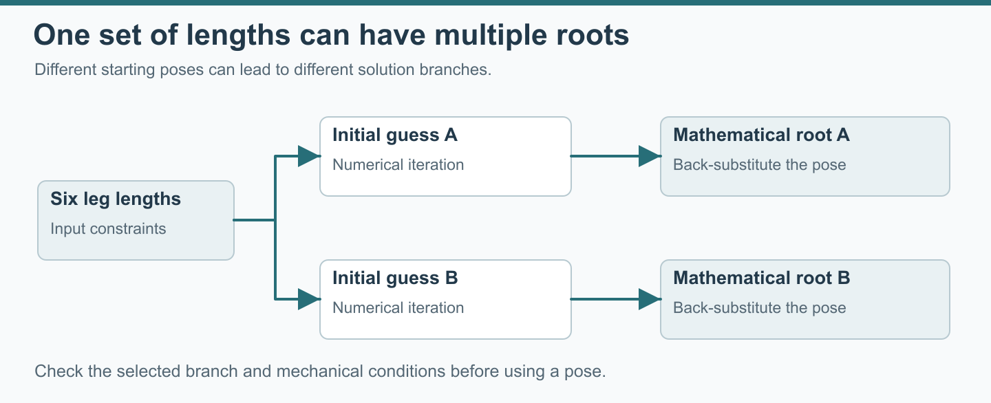
Forward kinematics starts with six leg lengths and seeks the moving plate’s position and orientation. The unknown pose appears inside all six distance equations. Changing one angle moves every upper attachment, so the equations must be solved together.
For measured or otherwise supplied lengths Lᵢ, define a length residual for a trial pose:
Scroll horizontally to read the full equation →
rᵢ(t, R) = ‖t + R pᵢ − bᵢ‖ − Lᵢ, for i = 1,…,6.
A solution makes all six residuals zero in the ideal model. With noisy or inconsistent inputs, a numerical method may instead minimize a weighted residual measure. Define the measurement model before choosing residual weights and acceptance tolerances.
The elimination-template study presents an algebraic method for the general problem and discusses specialized geometries. The practical difficulty is obtaining an appropriate solution efficiently, while distinguishing mathematical roots from configurations that the mechanism can actually occupy.
Six distances do not automatically identify one usable pose
Different assembly configurations can satisfy the same length constraints. An especially simple illustration uses the planar attachment geometry above: at R = I, changing the neutral translation from (0, 0, 400) to (0, 0, −400) leaves every squared distance unchanged. The lower configuration is a mathematical solution of that ideal distance model; it is not an operating position.
More generally, a root finder does not know the intended branch merely because the input contains six lengths. The operating configuration, allowable region, continuity from a known pose, and any additional relevant measurements help determine which solution is acceptable. Review other possible roots separately when selecting an assembly branch.
Understand what the local Jacobian does
Let uᵢ = sᵢ/lᵢ be the unit vector along a leg and aᵢ = R pᵢ the upper attachment offset from the moving-frame origin, expressed in base coordinates. For origin linear velocity v and angular velocity ω in the base frame, the leg rate is:
Scroll horizontally to read the full equation →
l̇ᵢ = uᵢᵀv + (aᵢ × uᵢ)ᵀω
Stacking six rows gives l̇ = J [vᵀ, ωᵀ]ᵀ. The Jacobian relates small motions or velocities about the current configuration; it is not a substitute for the full finite-rotation equation. The Jacobian discussion develops this local relationship.
Angular velocity components are not generally the same as roll, pitch, and yaw rates. If a solver updates Euler angles, its derivatives must include the chosen angle convention. A matrix built for a spatial rotation increment cannot be used unchanged as an Euler-angle derivative matrix.
Near a singular configuration, the local relationship can lose rank or become poorly conditioned. Numerical regularization changes the update calculation; geometric constraints still govern the mechanism. Translation and angular coordinates also use different units, so matrix scaling matters when interpreting conditioning.
Check the returned pose by going forward through the distance model
A practical numerical solve begins with an estimated pose, computes length residuals, updates the estimate, and repeats subject to limits. For the teaching example, a local solve initialized at the reference pose returns approximately t = (10, −5, 420) mm and (roll, pitch, yaw) = (5°, −3°, 8°) when given the unrounded target lengths.
The independent Python verification recovered the target pose and recomputed all six lengths. The maximum back-substitution residual was 5.684 × 10⁻¹⁴ mm, close to floating-point zero. That is floating-point agreement in an ideal model, not a property of a physical platform. To review your own result, retain the input lengths, initial pose, rotation convention, stopping conditions, final pose, and six recomputed lengths. Check both residual size and whether the answer stays on the intended branch. Compare unrounded values; rounding a table before solving introduces a different input dataset.
How Production Controllers Combine a Learned Initial Guess and Numerical Iteration
A neural network can provide an initial pose estimate, while a numerical method refines that estimate against the geometric equations. These stages have different responsibilities. The first predicts a useful starting point; the second checks and reduces inconsistency with the supplied lengths and geometry.
One published hybrid forward-kinematics study combines a learned initial estimate, numerical refinement, and prediction from motion history. It illustrates the general approach; implementations differ.
CSCmotion uses a neural-network initial guess followed by numerical iteration for forward kinematics in its production controllers. The engineering significance is the separation between a starting estimate and a solution checked against the geometric relationship. Check project-level controller requirements against the agreed configuration and interface.
A result that appears plausible still needs to be interpreted within the intended platform geometry and operating configuration. The six lengths alone do not explain which physical assembly branch is in use. A useful engineering discussion therefore connects the returned pose to the actual configuration and the meaning of the feedback supplied to the host.
For a buyer integrating a research system, the relevant deliverable is a clear interface and a documented interpretation of its fields. Confirm which values are commanded, which are measured directly, and which are reconstructed from a model. If an experiment requires an independent observation of the plate, define that measurement separately instead of treating a calculated pose as external evidence.
The synthetic verification above uses a conventional local numerical solve from a reference pose. It does not reproduce the production initializer.
Checking Your Model Against a Real Platform
Begin with the geometry and measurement definitions, then compare motion. After an internal consistency check, compare attachment coordinates, zero references, and calculated pose with the physical platform.
Compare engineering inputs before hardware testing.
Scroll horizontally to view all columns →
| Review item | Information to compare | Why it affects the result |
|---|---|---|
| Attachment geometry | Coordinates of all twelve joint centers, leg numbering, and units | A correct equation with the wrong pairing predicts another mechanism |
| Reference configuration | Plate origin, height, orientation, and definition of zero | Relative motion can be mistaken for an absolute pose |
| Rotation representation | Axis directions, order, angle units, and frame mapping | Identical angle labels can represent different spatial rotations |
| Actuator readings | Relationship between sensor output and joint-center length | Motor or encoder position may include offsets and transmission factors |
| Mechanical envelope | Actuator stroke, joint angular travel, and clearance constraints | Check clearance with all six legs in the requested pose |
| Motion path | Intermediate poses and associated rates | Evaluate the intermediate path as well as its endpoints |
| Independent comparison | External reference measurement and its coordinate alignment | Model-derived pose feedback is not independent evidence of plate pose |
Separate the geometric model from the motion response
A pose trajectory can be converted into six leg-position trajectories before a controller drives a simulated mechanism. The official pose-to-leg trajectory example illustrates this separation. The inverse solution specifies requested geometry; a dynamic model describes the motor, drive, and loaded mechanism response over time.
Payload weight, center of gravity, inertia, structural stiffness, and force requirements are additional inputs when evaluating a real motion system. Evaluate those inputs in the mechanical and dynamic model alongside the geometric distance calculation.
Likewise, position, velocity, and acceleration describe different aspects of a trajectory. A sequence of reachable positions can still demand leg rates or dynamic behavior that the selected platform has not been shown to deliver. Compare the required leg rates with the project motion requirements.
Use diagnostic examples that isolate a definition
Start by comparing the documented reference pose in both models. Then examine a small translation or rotation using the agreed coordinate convention. Finally, compare a mixed pose such as the teaching example. This progression makes it easier to identify whether a difference begins with an offset, a sign, a rotation order, or a leg connection.
For an analytical comparison, keep the same unrounded geometry in both calculations. For a comparison with measured hardware, also retain the origin of each measurement and the conversion used. Do not silently replace a measured joint-center location with an ideal circle simply because the ideal model is more convenient.
A platform may report pose computed from actuator encoder data through forward kinematics. CSCmotion’s available pose feedback follows that model-derived category. An external position or orientation measurement answers a different question and requires its own reference alignment and measurement conditions.
For each comparison, make a short calculation record with four columns: input definition, intermediate result, expected relationship, and observed difference. For leg geometry, the intermediate result is the transformed upper attachment point. For a length conversion, it is the joint-center distance after applying the documented offset. For a pose comparison, it is the coordinate transformation between the two measurement references.
This record helps localize a disagreement. If the transformed points already differ, investigate the coordinate or geometry inputs before the numerical solver. If points agree but lengths differ, compare the distance calculation and units. If geometric results agree while measured motion differs, retain the distinction and investigate the additional model or measurement assumptions.
Keep geometry revisions with those records. Changing an attachment coordinate, reference height, or calibration offset changes the mathematical problem, even when the software project name stays the same. Recalculate the comparison cases after such a change and identify which input set produced each result.
Read a residual as a statement about the calculation
There are two different comparisons in the numerical result. First, the recovered pose is compared with the original pose used to generate the target lengths. That comparison is possible because this is a synthetic example with known inputs. Second, the recovered pose is substituted into the leg-length equations and compared with the supplied target lengths. The latter checks satisfaction of the equations.
In a laboratory, the original physical pose may be unknown. A small residual can coexist with a systematic offset shared by the geometry and length conversion. Recording the source of the input data is therefore as important as recording the final residual.
Displayed decimal places also need careful interpretation. The tables round coordinates and lengths so a reader can inspect them. A calculation that starts from the rounded table is solving a slightly different problem from one that starts from the defining radii and angles. Use the defining inputs for reproduction; use the rounded values for a quick reasonableness check.
An unsuccessful local solve is informative too. Keep the supplied lengths and the initial estimate together so another reviewer can reproduce the same attempt. Before changing the model, check whether the inputs refer to the same geometry revision and reference configuration. Keep solver adjustments separate from physical calibration and host-interface revisions.
Carry the assumptions into the project handoff
For research motion platforms, a useful handoff identifies the scientific task, the platform coordinate definition, desired trajectories, payload information, feedback channels, and the comparison method. Explain whether the experiment needs commanded pose, reconstructed pose, or an independently measured motion variable.
Simulation software and hardware interfaces should share the same units and meaning for each field. During software integration, explicitly distinguish an absolute reference from an incremental displacement. Retain that distinction in data files and plots so that two traces with similar labels are not compared as if they represented the same quantity.
Use the motion platform selection checklist to assemble the load case and motion requirements. The related 6DOF motion platforms page addresses the complete platform discussion. For the distinction between naming and application requirements, compare hexapod vs Stewart platform.
FAQ
Does a Stewart platform always have six degrees of freedom?
A conventional spatial Stewart platform is intended to control three translations and three rotations. Six legs alone do not prove six independent controllable motions for every layout and pose. Joint architecture, geometric constraints, and singular configurations matter. A planar teaching mechanism may use fewer variables and legs; its equations cannot be transferred directly to a spatial hexapod without rebuilding the model.
Are Stewart platform equations of motion the same as kinematics equations?
Kinematics describes the geometry and rates of motion. Dynamic equations also relate motion to forces, torques, mass, inertia, and other modeled effects. If the task is dynamic modeling and simulation of a Stewart platform, first confirm the kinematics, then define the additional mechanical and control assumptions needed for that task.
Can I use these equations in MATLAB or Simulink?
The distance relationship is independent of a particular software environment. A MATLAB/Simulink or other modeling workflow still needs explicit attachment geometry, units, rotation order, and a reference configuration. Use the worked values to compare calculations before treating a model as a representation of hardware.
Is the calculated leg length the required actuator stroke?
No. Joint-center length is the total distance between the two attachment points. Required displacement is a difference between configurations; required stroke depends on the range of lengths across the intended motion and the actual actuator assembly. Check intermediate poses as well as endpoints.
Can six encoder readings prove the platform pose?
Six calibrated length inputs can support a forward-kinematics estimate when geometry, reference definitions, and the intended assembly branch are known. Encoder readings must first be related to those lengths. The resulting estimate remains dependent on the model. To compare it with actual plate motion, use an appropriate independent measurement and account for its reference frame and conditions.
Why can a model pass a neutral-pose check and fail after rotation?
At a neutral pose, some rotation-convention differences or geometry symmetries can be hidden. A mixed pose makes the transformations interact. Compare the upper attachment coordinates after rotation, then after translation, and finally the six leg vectors. This intermediate comparison is more informative than changing solver settings until the final lengths happen to look similar.
References
- Kinematic study of a Stewart platform: leg geometry and local Jacobian.
- General Stewart–Gough forward kinematics using elimination templates, a research preprint.
- Hybrid forward kinematics using a learned estimate and numerical refinement, Actuators, 2025.
- Pose-trajectory and leg-position simulation example.
Discussing a platform requirement
CSCmotion supplies complete electric motion platforms and develops its own platform kinematics and control technology. All platforms are custom, based on the customer’s load, stroke, speed and acceleration; there are no standard catalog models. CSCmotion 6DOF platforms use Cardan joints. For Stewart platforms built around a project load case, prepare the payload, coordinate definition, motion trajectory, interface needs, and verification requirements for engineering review.
Discuss your project with CSCmotion. Share your application, moving load and required motion for a free feasibility review and quotation.